The K-pototypes algorithm combines the K-means method with the K-modes method that can be used to process symbol attributes according to the K-means method. Compared with the K-means method, the K-pototypes algorithm can handle symbol attributes.
CLARANS algorithm (division method)CLARANS algorithm is a random search clustering algorithm, which is a segmentation clustering method. It first randomly selects a point as the current point, and then randomly checks some neighboring points around it that do not exceed the parameter Maxneighbor. If a better neighboring point is found, then it is moved to the neighboring point, otherwise the point is taken as Local minimum amount. Then randomly select a point to find another local minimum amount until the number of local minimums found reaches the user's requirements. The algorithm requires that the clustered objects must be pre-tuned to the memory, and the data set needs to be scanned multiple times. This is quite large for both large data volume and time complexity and space complexity. Although the performance of the R-tree structure is improved to enable it to handle large disk-based databases, the construction and maintenance of R*-trees is too costly. The algorithm is not sensitive to dirty data and abnormal data, but is extremely sensitive to the data object order, and can only deal with convex or spherical boundary clustering.
BIRCH algorithm (hierarchical method)The BIRCH algorithm is the balanced iterative reduction clustering method. The core of the method is to use a clustering feature 3-tuple to represent the information of a cluster, so that the representation of a cluster of points can be used with corresponding clustering features without having to use a specific set of points. To represent. It clusters by constructing a clustering feature tree that satisfies the branching factor and cluster diameter limits. The BIRCH algorithm can conveniently perform center, radius, diameter, and intra-class and inter-class distance calculations through clustering features. The clustering feature tree of the algorithm is a highly balanced tree with two parameter branching factors B and a class diameter T. The branching factor specifies the maximum number of children in each node of the tree, and the class diameter reflects the limitation on the diameter of a class of points, that is, the extent to which these points can be grouped into one class, and the non-leaf nodes are its The children's largest keywords can be indexed based on these keywords, which summarizes the information of their children.
The clustering feature tree can be constructed dynamically, so all data is not required to read the memory, but can be read one by one on the external memory. The new data item is always inserted into the tree in the tree closest to the data. If the diameter of the leaf is larger than the class diameter T after insertion, the leaf node is split. Other leaf nodes also need to check whether the branching factor is exceeded to determine whether it is split or not until the data is inserted into the leaf and does not exceed the class diameter, and the number of children of each non-leaf node is not greater than the branching factor. The algorithm can also modify the feature tree size by changing the class diameter to control its memory capacity.
The BIRCH algorithm can perform better clustering by one scan, which shows that the algorithm is suitable for large data volume. For a given M megabyte of memory space, the space complexity is O(M) and the inter-time complexity is O(dNBlnB(M/P)). Where d is the dimension, N is the number of nodes, P is the size of the memory page, and B is the branching factor determined by P. I/O costs are linear with the amount of data. The BIRCH algorithm is only applicable to the case where the distribution of the class is convex and spherical, and because the BIRCH algorithm needs to provide correct cluster number and cluster diameter limit, it is not feasible for invisible high-dimensional data.
CURE algorithm (hierarchical method)The CURE algorithm uses a clustering method that represents points. The algorithm first treats each data point as a class and then merges the nearest class until the number of classes is the required number. The CURE algorithm improves the traditional representation of classes, avoids using all points or using centers and radii to represent a class, but extracts a fixed number of well-distributed points from each class as a representative of this class. Point and multiply these points by an appropriate shrink factor to bring them closer to the center point of the class. A class is represented by a representative point such that the extension of the class can be extended to a non-spherical shape so that the shape of the class can be adjusted to express those non-spherical classes. In addition, the use of shrinkage factors reduces the effect of arpeggios on clustering. The CURE algorithm uses a combination of random sampling and segmentation to improve the spatial and temporal efficiency of the algorithm, and uses the heap and Kd tree structure to improve the efficiency of the algorithm.
DBSCAN algorithm (density based method)The DBSCAN algorithm is a density-based clustering algorithm. The algorithm uses the density connectivity of classes to quickly find classes of arbitrary shapes. The basic idea is that for each object in a class, the object contained in the field of its given radius cannot be less than a given minimum number. In the DBSCAN algorithm, the process of discovering a class is based on the fact that a class can be determined by any of the core objects. In order to find a class, DBSCAN first finds any object P from the object set D, and finds all objects in D that are reachable from the P density with respect to the diameter Eps and the minimum number of objects Minpts. If P is the core object, that is, the object contained in the neighborhood of P with radius Eps is not less than Minpts, according to the algorithm, a class about parameters Eps and Minpts can be found. If P is a boundary point, the P neighborhood with a radius of Eps contains fewer objects than Minpts, and P is temporarily labeled as a noise point. Then, DBSCAN processes the next object in D.
The acquisition of density-reachable objects is achieved by continuously performing regional queries. A region query returns all objects in the specified region. In order to efficiently perform regional queries, the DBSCAN algorithm uses a spatial query R-tree structure. Before performing clustering, an R*-tree must be established for all data. In addition, DBSCAN requires the user to specify a global parameter Eps (in order to reduce the amount of calculation, the parameters Minpts are predetermined). To determine the value, DBSCAN calculates the distance between any object and its kth nearest object. Then, according to the obtained distance, the order is sorted from small to large, and the sorted graph is drawn, which is called k-dist graph. The abscissa in the k-dist graph represents the distance between the data object and its kth nearest object; the ordinate is the number of data objects corresponding to a certain k-dist distance value. The establishment of the R*-tree and the drawing of the k-dist map are very time consuming. In addition, in order to obtain better clustering results, the user must select a suitable Eps value by heuristics according to the k-dist graph. The DBSCAN algorithm performs clustering operations on the entire data set without any pre-processing. When the amount of data is very large, there must be a large amount of memory support, and I/O consumption is also very large. The time complexity is O(nlogn) (n is the amount of data), and most of the clustering process is used in the area query operation. The DBSCAN algorithm is very sensitive to the parameters Eps and Minpts, and these two parameters are difficult to determine.
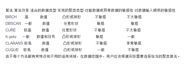
CLIQUE algorithm (combined with density-based and grid-based algorithms)The CLIQUE algorithm is an automatic subspace clustering algorithm. The algorithm uses the top-up method to find the clustering units of each subspace. The CLUQUE algorithm is mainly used to find low-dimensional clusters that exist in high-dimensional data space. In order to find the d-dimensional spatial clustering, it is necessary to combine the clusters of all d-1 dimensional subspaces, resulting in low spatial and temporal efficiency of the algorithm, and requires the user to input two parameters: the data value space is equally spaced. Distance and density are wide. These two parameters are closely related to the sample data, and users are generally difficult to determine. The CLIQUE algorithm is not sensitive to the order in which data is entered.
Based on the above analysis, we obtain the comparison results of each clustering algorithm, and the conclusions are as follows:
The K-means algorithm should be the most basic but also the most important algorithm in clustering algorithms. The algorithm flow is as follows:
Randomly take k points as k initial centroids;
Calculate the distance from other points to the k centroids;
If a point p is closer to the nth centroid, the point belongs to cluster n and is labeled, labeled point p.label=n, where n "=k;
Calculate the average of the point vectors in the same cluster, which is the same label, as the new centroid;
Iterate until all centroids do not change, ie the algorithm ends.
Of course, there are many ways to implement the algorithm. For example, when selecting the initial centroid, you can randomly select k, or you can randomly select k points that are farthest away, etc., and the methods are not the same.
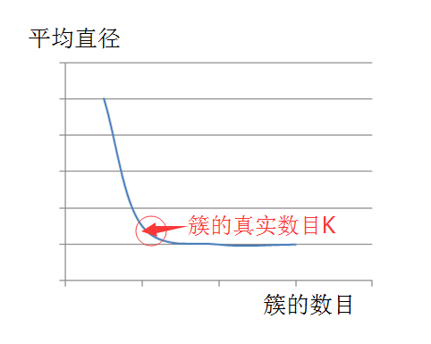
K value estimateFor k values, you must know ahead of time, which is also a disadvantage of the kmeans algorithm. Of course, for k values, we can have a variety of methods to estimate. In this paper, we use the average diameter method to estimate k.
That is, first consider all points as a large overall cluster, and calculate the average of the distances between all points as the average diameter of the cluster. When selecting the initial centroid, first select the two farthest points, and then start from the two most points, the point far from the two most points (the farthest degree is that the point is the most selected before) The distance between the two far points is greater than the average diameter of the overall cluster. It can be regarded as the newly discovered centroid, otherwise it will not be regarded as the centroid. Imagine if you use the average radius or average diameter indicator, if we guess the K value is greater than or equal to the true K value, which is the true number of clusters, then the upward trend of the indicator will be slow, but if we give When the K value is smaller than the number of real clusters, this indicator will definitely rise sharply.
Based on this estimation idea, we can estimate the correct k value and get k initial centroids. Then, we continue to iterate according to the above algorithm flow until all the centroids do not change, thus successfully implementing the algorithm. As shown below:
Figure 1. K-value estimate
We know that the k-means always converge, that is, the k-means algorithm must reach a steady state, in which all points are not transferred from one cluster to another, so the centroid does not change. Here, we introduce a pruning optimization, that is, the convergence process with the most obvious k-means will occur in the early stage of the algorithm. Therefore, in some cases, in order to increase the efficiency of the algorithm, we can replace the fifth step of the above algorithm. , using "iteration to only 1% to 3% of points affecting the centroid" or "iteration to only 1% to 3% of the point in the cluster".
The k-means apply to most data types and are simple and effective. But its shortcoming is that you need to know the exact k value, and can not handle the heterogeneous clusters, such as spherical clusters, clusters of different sizes and densities, ring clusters, and so on.
This article mainly explains and implements the algorithm. Therefore, the code implementation does not consider object-oriented thinking for the time being. It adopts the process-oriented implementation. If the data is multi-dimensional, it may need to do data preprocessing, such as normalization, and modify the code related method.
Algorithm implementationListing 1. Kmeans algorithm code implementation
Import java.io.BufferedReader;
Import java.io.FileReader;
Import java.io.IOException;
Import java.io.PrintStream;
Import java.text.DecimalFormat;
Import java.util.ArrayList;
Import java.util.Comparator;
Import java.util.PriorityQueue;
Import java.util.Queue;
Public class Kmeans {
Private class Node {
Int label;// label is used to record points belonging to the first cluster
Double[] attributes;
Public Node() {
Attributes = new double[100];
}
}
Private class NodeComparator {
Node nodeOne;
Node nodeTwo;
Double distance;
Public void compute() {
Double val = 0;
For (int i = 0; i " dimension ; ++i ) {
Val += (this.nodeOne.attributes[i] - this.nodeTwo.attributes[i]) *
(this.nodeOne.attributes[i] - this.nodeTwo.attributes[i]);
}
This.distance = val;
}
}
Private ArrayList "Node" arraylist;
Private ArrayList "Node" centroidList;
Private double averageDis;
Private int dimension;
Private Queue "NodeComparator" FsQueue =
New PriorityQueue "NodeComparator" (150, / / ​​used to sort the distance between any two points, from large to small
New Comparator "NodeComparator" () {
Public int compare(NodeComparator one, NodeComparator two) {
If (one.distance "two.distance)
Return 1;
Else if (one.distance 》 two.distance)
Return -1;
Else
Return 0;
}
});
Public void setKmeansInput(String path) {
Try {
BufferedReader br = new BufferedReader(new FileReader(path));
String str;
String[] strArray;
Arraylist = new ArrayList "Node" ();
While ((str = br.readLine()) != null) {
strArray = str.split(",");
Dimension = strArray.length;
Node node = new Node();
For (int i = 0; i " dimension ; ++i ) {
Node.attributes[i] = Double.parseDouble(strArray[i]);
}
Arraylist.add(node);
}
Br.close();
} catch (IOException e) {
e.printStackTrace();
}
}
Public void computeTheK() {
Int cntTuple = 0;
For (int i = 0; i " arraylist.size() - 1; ++i) {
For (int j = i + 1; j " arraylist.size(); ++j) {
NodeComparator nodecomp = new NodeComparator();
nodecomp.nodeOne = new Node();
nodecomp.nodeTwo = new Node();
For (int k = 0; k " dimension ; ++k ) {
nodecomp.nodeOne.attributes[k] = arraylist.get(i).attributes[k];
nodecomp.nodeTwo.attributes[k] = arraylist.get(j).attributes[k];
}
Nodecomp.compute();
averageDis += nodecomp.distance;
FsQueue.add(nodecomp);
cntTuple++;
}
}
averageDis /= cntTuple;// Calculate the average distance
chooseCentroid(FsQueue);
}
Public double getDistance(Node one, Node two) {// Calculate the Euclidean distance between two points
Double val = 0;
For (int i = 0; i " dimension ; ++i ) {
Val += (one.attributes[i] - two.attributes[i]) * (one.attributes[i] - two.attributes[i]);
}
Return val;
}
Public void chooseCentroid(Queue "NodeComparator" queue) {
centroidList = new ArrayList "Node" ();
Boolean flag = false;
While (!queue.isEmpty()) {
Boolean judgeOne = false;
Boolean judgeTwo = false;
NodeComparator nc = FsQueue.poll();
If (nc.distance " averageDis)
Break; / / If the next tuple, the distance between the two nodes is less than the average distance, then do not continue iteration
If (!flag) {
centroidList.add(nc.nodeOne);// First join the two points that are the furthest away from all points
centroidList.add(nc.nodeTwo);
Flag = true;
} else {// After starting from the two farthest points that have been added before, find the point farthest from these two points,
// If the distance is greater than the average distance of all points, then the new centroid is considered to be found, otherwise it is not considered as the centroid
For (int i = 0; i " centroidList.size(); ++i) {
Node testnode = centroidList.get(i);
If (centroidList.contains(nc.nodeOne) || getDistance(testnode, nc.nodeOne) " averageDis) {
judgeOne = true;
}
If (centroidList.contains(nc.nodeTwo) || getDistance(testnode, nc.nodeTwo) " averageDis) {
judgeTwo= true;
}
}
If (!judgeOne) {
centroidList.add(nc.nodeOne);
}
If (!judgeTwo) {
centroidList.add(nc.nodeTwo);
}
}
}
}
Public void doIteration(ArrayList"Node" centroid) {
Int cnt = 1;
Int cntEnd = 0;
Int numLabel = centroid.size();
While (true) {// iterate until all centroids do not change
Boolean flag = false;
For (int i = 0; i " arraylist.size(); ++i) {
Double dis = 0x7fffffff;
Cnt = 1;
For (int j = 0; j " centroid.size(); ++j) {
Node node = centroid.get(j);
If (getDistance(arraylist.get(i), node) " dis) {
Dis = getDistance(arraylist.get(i), node);
Arraylist.get(i).label = cnt;
}
Cnt++;
}
}
Int j = 0;
numLabel -= 1;
While (j " numLabel) {
Int c = 0;
Node node = new Node();
For (int i = 0; i " arraylist.size(); ++i) {
If (arraylist.get(i).label == j + 1) {
For (int k = 0; k " dimension ; ++k ) {
Node.attributes[k] += arraylist.get(i).attributes[k];
}
c++;
}
}
DecimalFormat df = new DecimalFormat("#.###");// Keep three decimal places
Double[] attributelist = new double[100];
For (int i = 0; i " dimension ; ++i ) {
Attributelist[i] = Double.parseDouble(df.format(node.attributes[i] / c));
If (attributelist[i] != centroid.get(j).attributes[i]) {
Centroid.get(j).attributes[i] = attributelist[i];
Flag = true;
}
}
If (!flag) {
cntEnd++;
If (cntEnd == numLabel) {// If all centroids are unchanged, then jump out of the loop
Break;
}
}
j++;
}
If (cntEnd == numLabel) {// If all centroids are the same, then success
System.out.println("run kmeans successfully.");
Break;
}
}
}
Public void printKmeansResults(String path) {
Try {
PrintStream out = new PrintStream(path);
computeTheK();
doIteration(centroidList);
Out.println("There are †+ centroidList.size() + "cluster!");
For (int i = 0; i " arraylist.size(); ++i) {
Out.print("(");
For (int j = 0; j " dimension - 1; ++j) {
Out.print(arraylist.get(i).attributes[j] + ", ");
}
Out.print(arraylist.get(i).attributes[dimension - 1] + ") â€);
Out.println("belongs to cluster" + arraylist.get(i).label);
}
Out.close();
System.out.println("Please check results in: †+ path);
} catch (IOException e) {
e.printStackTrace();
}
}
Public static void main(String[] args) {
Kmeans kmeans = new Kmeans();
kmeans.setKmeansInput("c:/kmeans.txt");
kmeans.printKmeansResults("c:/kmeansResults.txt");
}
}
Test DataGive a simple set of 2D test data:
Listing 2. Kmeans algorithm test data
1,1
2,1
1,2
2,2
6,1
6,2
7,1
7,2
1,5
1,6
2,5
2,6
6,5
6,6
7,5
7,6
operation resultListing 3. Kmeans algorithm running results
There are 4 clusters!
(1.0, 1.0) belongs to cluster 1
(2.0, 1.0) belongs to cluster 1
(1.0, 2.0) belongs to cluster 1
(2.0, 2.0) belongs to cluster 1
(6.0, 1.0) belongs to cluster 3
(6.0, 2.0) belongs to cluster 3
(7.0, 1.0) belongs to cluster 3
(7.0, 2.0) belongs to cluster 3
(1.0, 5.0) belongs to cluster 4
(1.0, 6.0) belongs to cluster 4
(2.0, 5.0) belongs to cluster 4
(2.0, 6.0) belongs to cluster 4
(6.0, 5.0) belongs to cluster 2
(6.0, 6.0) belongs to cluster 2
(7.0, 5.0) belongs to cluster 2
(7.0, 6.0) belongs to cluster 2
Detailed analysis of hierarchical clustering algorithm and implementation of hierarchical clusteringHierarchical clustering is divided into cohesive hierarchical clustering and split hierarchical clustering.
Condensed hierarchical clustering means that each point is treated as a cluster in the initial stage, and then the two closest clusters are merged each time. Of course, the definition of the degree of proximity needs to specify the neighboring criterion of the cluster.
Split-level hierarchical clustering means that all points are treated as a cluster in the initial stage, and then one cluster is split each time until a cluster of single points is left.
In this article we will detail the condensed hierarchical clustering algorithm.
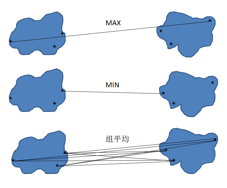
For condensed hierarchical clustering, specifying the cluster's proximity criterion is a very important part. Here we introduce the three most commonly used criteria, namely MAX, MIN, and group averaging. As shown below:
Figure 2. Hierarchical clustering calculation criteria
The condensed hierarchical clustering algorithm is also an iterative process. The algorithm flow is as follows:
Each time the next two clusters are merged, we will refer to these two merged clusters as merge clusters.
If the MAX criterion is used, the distance between the other clusters and the two points farthest from the merged cluster is selected as the proximity between the clusters. If the MIN criterion is used, the distance between the other clusters and the two closest points in the merged cluster is taken as the proximity between the clusters. If the group average criterion, the average of the distances between other clusters and all points of the merged cluster is taken as the proximity between the clusters.
Repeat steps 1 and 2 to merge until there is only one cluster left.
Algorithm process exampleLet's look at an example:
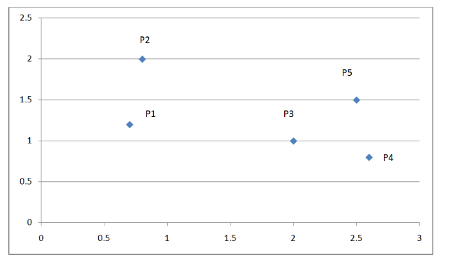
The figure below is a coordinate system with five points:
Figure 3. Example of hierarchical clustering
The following table shows the Euclidean distance matrix for these five points:
Table 1. Euclidean distance original matrix
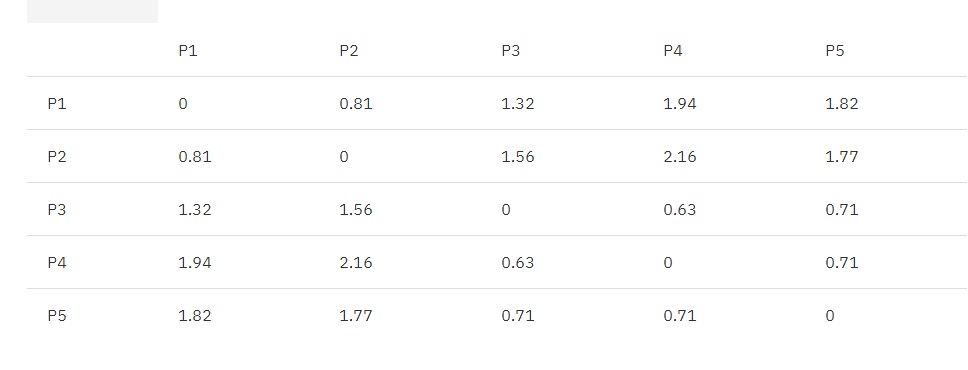
According to the algorithm flow, we first find the two clusters closest to each other, P3, P4.
Combine P3, P4 is {P3, P4}, and update the matrix according to the MIN principle as follows:
MIN.distance({P3, P4}, P1) = 1.32;
MIN.distance({P3, P4}, P2) = 1.56;
MIN.distance({P3, P4}, P5) = 0.70;
Table 2. Euclidean distance update matrix 1
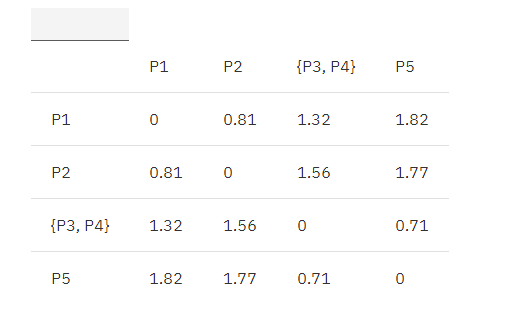
Then continue to find the two closest clusters, {P3, P4}, P5.
Combine {P3, P4}, P5 is {P3, P4, P5}, and continue to update the matrix according to the MIN principle:
MIN.distance(P1, {P3, P4, P5}) = 1.32;
MIN.distance(P2, {P3, P4, P5}) = 1.56;
Table 3. Euclidean distance update matrix 2
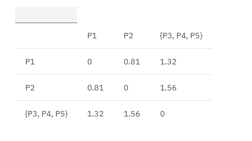
Then continue to find the nearest two clusters, P1, P2.
Combine P1, P2 is {P1, P2}, and continue to update the matrix according to the MIN principle:
MIN.distance({P1,P2}, {P3, P4, P5}) = 1.32
Table 4. Euclidean distance update matrix 3
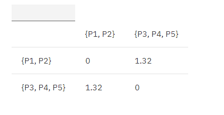
Finally, merge the remaining two clusters to get the final result, as shown below:
Figure 4. Example results for hierarchical clustering
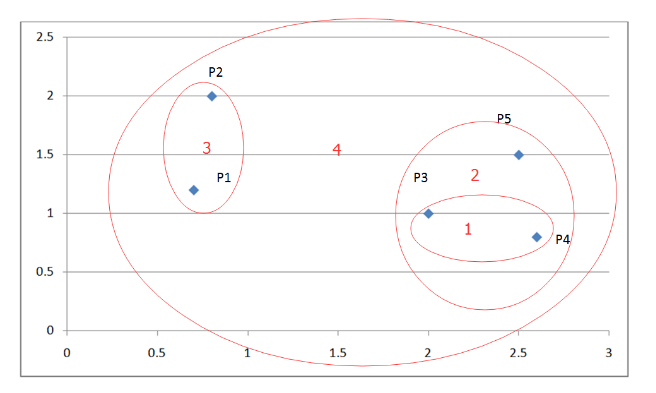
MAX, the group average algorithm flow is the same, except that when calculating the matrix, the distance between the calculated clusters is changed to the maximum Euclidean distance between the two points between the clusters, and the average Euclidean distance of all the points between the clusters is sufficient.
Algorithm implementationListing 4. Hierarchical clustering algorithm code implementation
Import java.io.BufferedReader;
Import java.io.FileReader;
Import java.io.IOException;
Import java.io.PrintStream;
Import java.text.DecimalFormat;
Import java.util.ArrayList;
Public class Hierarchical {
Private double[][] matrix;
Private int dimension;// data dimension
Private class Node {
Double[] attributes;
Public Node() {
Attributes = new double[100];
}
}
Private ArrayList "Node" arraylist;
Private class Model {
Int x = 0;
Int y = 0;
Double value = 0;
}
Private Model minModel = new Model();
Private double getDistance(Node one, Node two) {// Calculate the Euclidean distance between two points
Double val = 0;
For (int i = 0; i " dimension ; ++i ) {
Val += (one.attributes[i] - two.attributes[i]) * (one.attributes[i] - two.attributes[i]);
}
Return Math.sqrt(val);
}
Private void loadMatrix() {// Convert input data to matrix
For (int i = 0; i "matrix.length; ++i) {
For (int j = i + 1; j "matrix.length; ++j) {
Double distance = getDistance(arraylist.get(i), arraylist.get(j));
Matrix[i][j] = distance;
}
}
}
Private Model findMinValueOfMatrix(double[][] matrix) {// Find the nearest two clusters in the matrix
Model model = new Model();
Double min = 0x7fffffff;
For (int i = 0; i "matrix.length; ++i) {
For (int j = i + 1; j "matrix.length; ++j) {
If (min 》 matrix[i][j] && matrix[i][j] != 0) {
Min = matrix[i][j];
Model.x = i;
Model.y = j;
Model.value = matrix[i][j];
}
}
}
Return model;
}
Private void processHierarchical(String path) {
Try {
PrintStream out = new PrintStream(path);
While (true) {// condensed hierarchical clustering iteration
Out.println("Matrix update as below: ");
For (int i = 0; i "matrix.length; ++i) {// Output the matrix updated every iteration
For (int j = 0; j " matrix.length - 1; ++j) {
Out.print(new DecimalFormat("#.00").format(matrix[i][j]) + " ");
}
Out.println(new DecimalFormat("#.00").format(matrix[i][matrix.length - 1]));
}
Out.println();
minModel = findMinValueOfMatrix(matrix);
If (minModel.value == 0) {// When the two clusters closest to the distance are not found, the iteration ends.
Break;
}
Out.println("Combine" + (minModel.x + 1) + " " + (minModel.y + 1));
Out.println("The distance is: " + minModel.value);
Matrix[minModel.x][minModel.y] = 0;// Update matrix
For (int i = 0; i "matrix.length; ++i) {// If the points p1 and p2 are merged, only one of p1 and p2 is reserved from other points, whichever is smaller
If (matrix[i][minModel.x] <<= matrix[i][minModel.y]) {
Matrix[i][minModel.y] = 0;
} else {
Matrix[i][minModel.x] = 0;
}
If (matrix[minModel.x][i] <<= matrix[minModel.y][i]) {
Matrix[minModel.y][i] = 0;
} else {
Matrix[minModel.x][i] = 0;
}
}
}
Out.close();
System.out.println("Please check results in: †+ path);
} catch (Exception e) {
e.printStackTrace();
}
}
Public void setInput(String path) {
Try {
BufferedReader br = new BufferedReader(new FileReader(path));
String str;
String[] strArray;
Arraylist = new ArrayList "Node" ();
While ((str = br.readLine()) != null) {
strArray = str.split(",");
Dimension = strArray.length;
Node node = new Node();
For (int i = 0; i " dimension ; ++i ) {
Node.attributes[i] = Double.parseDouble(strArray[i]);
}
Arraylist.add(node);
}
Matrix = new double[arraylist.size()][arraylist.size()];
loadMatrix();
Br.close();
} catch (IOException e) {
e.printStackTrace();
}
}
Public void printOutput(String path) {
processHierarchical(path);
}
Public static void main(String[] args) {
Hierarchical hi = new Hierarchical();
hi.setInput("c:/hierarchical.txt");
hi.printOutput("c:/hierarchical_results.txt");
}
}
Test DataGive a simple set of 2D test data
Listing 5. Hierarchical clustering algorithm test data
0.7, 1.2
0.8, 2
2,1
2.6, 0.8
2.5, 1.5
operation resultListing 6. Hierarchical clustering algorithm run results
Matrix update as below:
.00 .81 1.32 1.94 1.82
.00 .00 1.56 2.16 1.77
.00 .00 .00 .63 .71
.00 .00 .00 .00 .71
.00 .00 .00 .00 .00
Combine 3 4
The distance is: 0.6324555320336759
Matrix update as below:
.00 .81 1.32 .00 1.82
.00 .00 1.56 .00 1.77
.00 .00 .00 .00 .00
.00 .00 .00 .00 .71
.00 .00 .00 .00 .00
Combine 4 5
The distance is: 0.7071067811865475
Matrix update as below:
.00 .81 1.32 .00 .00
.00 .00 1.56 .00 .00
.00 .00 .00 .00 .00
.00 .00 .00 .00 .00
.00 .00 .00 .00 .00
Combine 1 2
The distance is: 0.806225774829855
Matrix update as below:
.00 .00 1.32 .00 .00
.00 .00 .00 .00 .00
.00 .00 .00 .00 .00
.00 .00 .00 .00 .00
.00 .00 .00 .00 .00
Combine 1 3
The distance is: 1.3152946437965907
Matrix update as below:
.00 .00 .00 .00 .00
.00 .00 .00 .00 .00
.00 .00 .00 .00 .00
.00 .00 .00 .00 .00
.00 .00 .00 .00 .00
Detailed explanation and implementation of DBSCAN algorithmConsidering a situation where the distribution of points is not uniform and the shape is irregular, the Kmeans algorithm and the hierarchical clustering algorithm will face the risk of failure.
The following coordinate system:
Figure 5. DBSCAN algorithm example
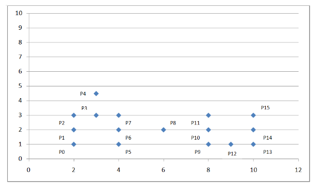
We can see that the dot density above is not uniform, then we consider a density-based clustering algorithm: DBSCAN.
Algorithm flowSet the scan radius Eps and specify the density value within the scan radius. If the density in the radius of the current point is greater than or equal to the set density value, set the current point as the core point; if a point is just on the radius edge of a certain core point, set this point as the boundary point; if a point is neither The core point is not a boundary point, then this point is a noise point.
Remove noise points.
All core points within the scan radius are assigned to the edges for communication.
Each set of connected core points is labeled as a cluster.
Assign all boundary points to the cluster total of the corresponding core points.
Algorithm process exampleAs shown in the coordinate system above, we set the scan radius Eps to 1.5 and the density threshold threshold to 3. Through the above algorithmic process, we can get the following figure:
Figure 6. Example DBCCAN algorithm example results
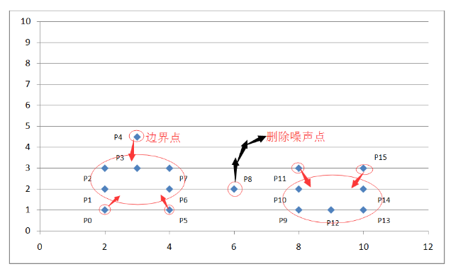
By calculating the Euclidean distance between each point and the density value within the scanning radius, it is judged that these points belong to the core point, the boundary point or the noise point. Because we set the scan radius to 1.5 and the density threshold to 3, so:
The P0 point is the boundary point because there are only two points P0 and P1 within the scanning radius centered on it;
The P1 point is the core point because there are four points P0, P1, P2, P4 in the scanning radius centered on it;
P8 is a noise point because it is neither a core point nor a boundary point;
Other points are analogous.
Algorithm implementationListing 7. DBSCAN algorithm code implementation
Import java.io.BufferedReader;
Import java.io.FileReader;
Import java.io.IOException;
Import java.io.PrintStream;
Import java.util.ArrayList;
Import java.util.HashMap;
Import java.util.Iterator;
Import java.util.Map;
Public class DBSCAN {
Private int dimension;// data dimension
Private double eps = 1.5;
Private int threshold = 3;
Private double distance[][];
Private Map "Integer, Integer" id = new HashMap "Integer, Integer" ();
Private int countClusters = 0;
Private ArrayList "Integer" keyPointList = new ArrayList "Integer" (); / /
Private int[] flags;// mark edge points
Private class Edge {
Int p, q;
Double weight;
}
Private class Node {
Double[] attributes;
Public Node() {
Attributes = new double[100];
}
}
Private ArrayList "Node" nodeList;
Private ArrayList "Edge" edgeList;
Private double getDistance(Node one, Node two) {// Calculate the Euclidean distance between two points
Double val = 0;
For (int i = 0; i " dimension ; ++i ) {
Val += (one.attributes[i] - two.attributes[i]) * (one.attributes[i] - two.attributes[i]);
}
Return Math.sqrt(val);
}
Public void loadEdges() {// Adds edges between all core points within the scan radius, marks the boundary points and automatically ignores the noise points
edgeList = new ArrayList "Edge" ();
Flags = new int[nodeList.size()];
Int[] countPoint = new int[nodeList.size()];
For (int i = 0; i " countPoint.length; ++i) {
countPoint[i] = 1;// Each point is a core point at the beginning
}
For (int i = 0; i " nodeList.size(); ++i) {
For (int j = i + 1; j " nodeList.size(); ++j) {
Distance[i][j] = getDistance(nodeList.get(i), nodeList.get(j));
If (distance[i][j] <<= eps) {// The distance between two points is less than the scan radius
countPoint[i]++;
If (countPoint[i] 》 0 && countPoint[i] "threshold" {
Flags[i] = j;// record boundary points
}
If (countPoint[i] 》= threshold) {// If the density value within the scan radius of the current point is recorded is greater than or equal to the given threshold
Flags[i] = 0;
If (!keyPointList.contains(i)) {
keyPointList.add(i);
}
}
countPoint[j]++;
If (countPoint[j] 》 0 && countPoint[j] threshold) {
Flags[j] = i;// record boundary points
}
If (countPoint[j] 》= threshold) {// If the density value within the scan radius of the current point is recorded is greater than or equal to the given threshold
Flags[j] = 0;
If (!keyPointList.contains(j)) {
keyPointList.add(j);
}
}
}
}
}
For (int i = 0; i " keyPointList.size(); ++i) {
For (int j = i + 1; j "keyPointList.size(); ++j) {
Edge edge = new Edge();
Edge.p = keyPointList.get(i);
Edge.q = keyPointList.get(j);
Edge.weight = distance[edge.p][edge.q];
If (edge.weight <<= eps) {
If (!id.containsKey(edge.p)) {// Prepare for later use and check for connected components
Id.put(edge.p, edge.p);
}
If (!id.containsKey(edge.q)) {
Id.put(edge.q, edge.q);
}
edgeList.add(edge);
}
}
}
}
Public void setInput(String path) {
Try {
BufferedReader br = new BufferedReader(new FileReader(path));
String str;
String[] strArray;
nodeList = new ArrayList "Node" ();
While ((str = br.readLine()) != null) {
strArray = str.split(",");
Dimension = strArray.length;
Node node = new Node();
For (int i = 0; i " dimension ; ++i ) {
Node.attributes[i] = Double.parseDouble(strArray[i]);
}
nodeList.add(node);
}
Distance = new double[nodeList.size()][nodeList.size()];
loadEdges();
Br.close();
} catch (IOException e) {
e.printStackTrace();
}
}
Public void union(int p, int q) {// and operate
Int a = find(p);
Int b = find(q);
If (a != b) {
Id.put(a, b);
}
}
Public int find(int p) {// check operation
If (p != id.get(p)) {
Id.put(p, find(id.get(p)));
}
Return id.get(p);
}
Public void processDBSCAN(String path) {
Try {
PrintStream out = new PrintStream(path);
Out.println("core point:" + keyPointList);
Out.println();
For (int i = 0; i "edgeList.size(); ++i) {
Out.println("core point(" + edgeList.get(i).p + " " +
The distance between edgeList.get(i).q + ") is: †+ edgeList.get(i).weight);
}
For (int i = 0; i "edgeList.size(); ++i) {
Union(edgeList.get(i).p, edgeList.get(i).q);// Use point and set to change the point set into connected component
}
Iterator "Integer" it = id.keySet().iterator();
While (it.hasNext()) {
Int key = it.next();
If (id.get(key) == key) {// Use and check to get the number of strongly connected components
++countClusters;
}
}
Out.println();
For (int i = 0; i " flags.length; ++i) {
If (flags[i] != 0) {
Out.println("point" + i + "belongs to point" + flags[i] + "cluster");
}
}
Out.println();
Out.println("The number of connected components by the core point is known to be:" + countClusters + "cluster");
Out.close();
System.out.println(“Please check results in: †+ path);
} catch (Exception e) {
e.printStackTrace();
}
}
public void printOutput(String path) {
processDBSCAN(path);
}
public static void main(String[] args) {
DBSCAN dbscan = new DBSCAN();
dbscan.setInput(“c:/dbscan.txtâ€ï¼‰;
dbscan.printOutput(“c:/dbscan_results.txtâ€ï¼‰;
}
}
测试数æ®æ¸…å•8. DBSCAN 算法测试数æ®
2,1
2,2
2,3
3,3
3,4.5
4,1
4,2
4,3
6,2
8,1
8,2
8,3
9,1
10,1
10,2
10,3
è¿è¡Œç»“果清å•9. DBSCAN 算法è¿è¡Œç»“æžœ
æ ¸å¿ƒç‚¹ä¸ºï¼š ï¼»1, 2, 3, 6, 7, 9, 10, 12, 13, 14ï¼½
æ ¸å¿ƒç‚¹ï¼ˆ1 2) 之间的è·ç¦»ä¸ºï¼š 1.0
æ ¸å¿ƒç‚¹ï¼ˆ1 3) 之间的è·ç¦»ä¸ºï¼š 1.4142135623730951
æ ¸å¿ƒç‚¹ï¼ˆ2 3) 之间的è·ç¦»ä¸ºï¼š 1.0
æ ¸å¿ƒç‚¹ï¼ˆ3 6) 之间的è·ç¦»ä¸ºï¼š 1.4142135623730951
æ ¸å¿ƒç‚¹ï¼ˆ3 7) 之间的è·ç¦»ä¸ºï¼š 1.0
æ ¸å¿ƒç‚¹ï¼ˆ6 7) 之间的è·ç¦»ä¸ºï¼š 1.0
æ ¸å¿ƒç‚¹ï¼ˆ9 10) 之间的è·ç¦»ä¸ºï¼š 1.0
æ ¸å¿ƒç‚¹ï¼ˆ9 12) 之间的è·ç¦»ä¸ºï¼š 1.0
æ ¸å¿ƒç‚¹ï¼ˆ10 12) 之间的è·ç¦»ä¸ºï¼š 1.4142135623730951
æ ¸å¿ƒç‚¹ï¼ˆ12 13) 之间的è·ç¦»ä¸ºï¼š 1.0
æ ¸å¿ƒç‚¹ï¼ˆ12 14) 之间的è·ç¦»ä¸ºï¼š 1.4142135623730951
æ ¸å¿ƒç‚¹ï¼ˆ13 14) 之间的è·ç¦»ä¸ºï¼š 1.0
连通点1 和点2
连通点1 和点3
连通点3 和点6
连通点3 和点7
连通点9 和点10
连通点9 和点12
连通点12 和点13
连通点12 和点14
点1ã€ç‚¹2ã€ç‚¹3ã€ç‚¹6ã€ç‚¹7 åŒå±žäºŽç°‡1
点9ã€ç‚¹10ã€ç‚¹12ã€ç‚¹13ã€ç‚¹14 åŒå±žäºŽç°‡2
点0 属于点1 所在的簇
点4 属于点3 所在的簇
点5 属于点6 所在的簇
点11 属于点10 所在的簇
点15 属于点14 所在的簇
ç”±æ ¸å¿ƒç‚¹è¿žé€šåˆ†é‡æ•°é‡å¾—知共有: 2 个簇
其他èšç±»ç®—法简介 BIRCH 算法Birch 是一ç§èƒ½å¤Ÿé«˜æ•ˆå¤„ç†å¤§æ•°æ®èšç±»çš„åŸºäºŽæ ‘çš„å±‚æ¬¡èšç±»ç®—æ³•ã€‚è®¾æƒ³è¿™æ ·ä¸€ç§æƒ…况,一个拥有大规模数æ®çš„æ•°æ®åº“,当这些数æ®è¢«æ”¾å…¥ä¸»å˜è¿›è¡Œèšç±»å¤„ç†æ—¶ï¼Œä¸€èˆ¬çš„èšç±»ç®—法则没有对应的高效处ç†èƒ½åŠ›ï¼Œè¿™æ—¶Birch 算法是最佳的选择。
Birth ä¸ä»…能够高效地处ç†å¤§æ•°æ®èšç±»ï¼Œå¹¶ä¸”能最å°åŒ–IO 花销。它ä¸éœ€è¦æ‰«æ全局数æ®å·²ç»çŽ°æœ‰çš„簇。
算法æµç¨‹èšç±»ç‰¹å¾CF=(N,LS,SS),其ä¸N 代表簇ä¸ç‚¹çš„个数,LS 代表簇ä¸ä»£è¡¨ç°‡ä¸å„点线性和,SS 代表簇ä¸å„点的平方和è·ç¦»ã€‚èšç±»ç‰¹å¾è¢«åº”用于CF æ ‘ä¸ï¼ŒCF æ ‘æ˜¯ä¸€ç§é«˜åº¦å¹³è¡¡æ ‘,它具有两个å‚æ•°ï¼šå¹³è¡¡å› åB 和簇åŠå¾„阈值T。其ä¸å¹³è¡¡å› åB 代表æ¯ä¸€ä¸ªéžå¶å节点最多能够引入B 个实体æ¡ç›®ã€‚
å¶å节点最多åªèƒ½åŒ…å«L 个实体æ¡ç›®ï¼Œå¹¶ä¸”它们具有å‰å‘åŽå‘æŒ‡é’ˆï¼Œè¿™æ ·å¯ä»¥å½¼æ¤é“¾æŽ¥èµ·æ¥ã€‚
æ ‘çš„å¤§å°å–决于簇åŠå¾„阈值T 的大å°ã€‚
ä»Žæ ¹èŠ‚ç‚¹å¼€å§‹ï¼Œé€’å½’æŸ¥æ‰¾ä¸Žè¦æ’入的数æ®ç‚¹è·ç¦»æœ€è¿‘çš„å¶å节点ä¸çš„实体æ¡ç›®ï¼Œé€’归过程选择最çŸè·¯å¾„。
比较上述计算出的数æ®ç‚¹ä¸Žå¶å节点ä¸å®žä½“æ¡ç›®é—´çš„最近è·ç¦»æ˜¯å¦å°å¶ç°‡åŠå¾„阈值T,å°äºŽåˆ™å¸æ”¶è¯¥æ•°æ®ç‚¹ã€‚å¦åˆ™æ‰§è¡Œä¸‹ä¸€æ¥ã€‚
判æ–当å‰æ¡ç›®æ‰€åœ¨çš„å¶èŠ‚点个数是å¦å°äºŽL,若å°äºŽåˆ™ç›´æŽ¥å°†è¯¥æ•°æ®ç‚¹æ’入当å‰ç‚¹ã€‚å¦åˆ™åˆ†è£‚å¶å节点,分裂过程是将å¶å节点ä¸è·ç¦»æœ€è¿œçš„两个实体æ¡ç›®å˜ä¸ºæ–°çš„两个å¶å节点,其他æ¡ç›®åˆ™æ ¹æ®è·ç¦»æœ€è¿‘原则é‡æ–°åˆ†é…到这两个新的å¶å节点ä¸ã€‚åˆ é™¤åŽŸæ¥çš„å¶å节点并更新CF æ ‘ã€‚
Greeen Touch 5A series touch monitors as follows: 15", 17", 18.5", 19", 21.5", 22", 23.6",resistive, 5-wi touch technology"
♦ Adopt AUO,LG,BOE international premium A+ grade original industrial LED screen.
♦ Regular size 15"-23.6",resistive,capacitive,infrared touch technologies are optional.♦ Stable and sensitive,no jumping points,no break points,no blind spots.
♦ Industrial metal front shell and black frame,durable and reliable.
♦ Good sealing performance,passed EMC anti-interference testing.
♦ Optional external mounting bracket and standard VESA mounting.
♦ Running 24 hours a day,support OEM/ODM services.

Open Frame Touch Monitor,Touch Display Monitor,LCD Touchscreen Monitor,Resistive Touch Screen Monitor,Open Frame Touch Screen Display,Touch Screen LCD Monitor Display
ShenZhen GreenTouch Technology Co.,Ltd , https://www.bbstouch.com